Evaluating Precipitation Options in HEC-HMS

Dr. Nelson

Overview

At this stage you have learned the basic modeling techniques in HMS. Now we will be dealing with the individual component of the modeling in greater detail. We will begin with the precipitation and we will analyze how different spatial and temporal precipitation models can be used, and the way HMS responds to all of them.

Our sensitivity studies will center around the Judy's Branch Watershed and you can use the same data as you did previously. We will use different precipitation methods as input and see how the output varies. You will perform the similar analysis with GSSHA (in the next assignment) and at the end you will compare the response of both HMS and GSSHA to different precipitation methods.

There are four rain gauge stations close to Judy's Branch Watershed namely Belleville Siu Research, Carlinville 2, Carlyle Reservoir and St Louis Airport. the first three stations are in Illinois and last one is in Missouri.

Station	Belleville Siu Research	Carlinville 2	Carlyle Reservoir	St Louis Airport
Latitude	38.56°	38.99°	38.76°	38.74°
Longitude	-89.86°	-89.89°	-89.67°	-90.25°
State	Illinois	Illinois	Illinois	Missouri
Observing Site	Belleville Siu Research, IL	Carlinville 2, IL	Carlyle Reservoir, IL	StL, Mo

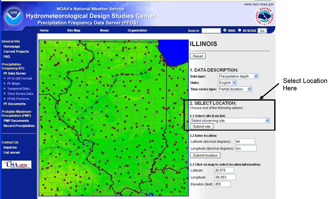
To get the frequency storm data, you need to go to NOAA Atlas 14 website. Then, select the state by clicking on the map. You can then choose the station name (Observing Site, see table above) by selecting from the drop down box. See the following Figure:

To get Daily and Hourly data, you can go to this NOAA page and download the data as *.pdf files. For this assignment we have compiled data from some "interesting" storms and prepared a spreadsheet with the data. 

Analysis

---

Go through following outlines of the assignment and try to understand the big picture of what you are going to do. Then go on to complete the Assignment

1. Basic Model set up:

• Delineate the Judy's Branch watershed again (or use from previous workshops).

• Import the land use and soil coverages

• Save this as your base modeling project.

• Set up a single basin HMS Model

  • CN = 99 (100 would be better, but HMS will not accept a CN of 100) 
    Calculate Ia (Here, we are using CN value of 99, try to figure out what this means and why are we trying to do this).

  • 24 hour storm duration

  • use the Clark Unit Hydrograph, with Tc and R calculated from Kerby method for overland flow

2. Precipitation Set up:

Here we will use various rainfall types (we are not going to analyze the snowmelt processes, so the term precipitation here will represent only the rainfall). We will be using the following rainfall methods.

To Examine Spatial Variation:

• Basin Average Precipitation method: we will use only one rain gauge station depth which we assume to be the representative of the entire watershed.

• Thiessen Polygon method for gauges:  we will use four different gauging stations (see table above for station details) and determine the basin average precipitation depths using  Thiessen Polygon area weighted average method. 

In order to use the Thiessen Polygon method in WMS:

• Add a new coverage in your WMS project and change its type to Rain gauge.

• Then select Create Feature Point tool and click somewhere over the watershed and edit the coordinates using the latitude longitude values given in the table above. Use the properties window at the right side of the WMS window to edit the coordinates of the gauges. Here you have to type the coordinates in decimal degrees.  Longitude values are negative because we are "west" of the prime meridian.

• Repeat the same process to enter other three stations. Then right click the rain gauge coverage and convert the coordinates from Geographic NAD 83 to UTM NAD 83, Zone 15 or 16 whichever you are using. This will bring the rain gauge stations in the proximity of watershed and WMS will automatically create Thiessen polygons.

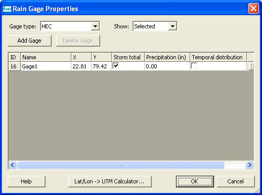
• After all the gauges are displayed in the right coordinate system, select Select Feature Object tool and double click on the gage icons. This will open up rain gage properties dialog where you can enter the depth, temporal distribution etc for the gage.

• You only need to define the temporal distribution for one of the gages.

• After defining the rain gage coverage you need to go to the HMS Meteorological model and define it to be gage weights. Then in define weights you must specify you are using the rain gage coverage (DO NOT Add gages here).

• Finally, you will need to compute the gage weights. This can be done by recomputing basin data or there is a specific command to compute gage weights, but it won't define the weights for HMS unless you have specified that you are using the rain gage coverage.  Accept the default grid size when prompted during these computations.

 

Examining Temporal Variations:

The temporal variation shows how the storm intensity changes over time, and the duration of the storm. For example if we know that a rainfall depth of 5 inches occurred in Belleville station between 5:00 AM and 7:00 AM, then the temporal distribution shows how the rainfall of 5 inches is distributed over the storm duration of 2 hours (5 am to 7am). This is an example of a 120 minute duration storm. On the other hand, the standard temporal distributions like Type I or II etc, distribute the rainfall over a period of 24 hours at an interval of 6 minutes.

The following temporal distributions will be analyzed:

• Type I distribution

• Type I a distribution

• Type II distribution

• Actual 60 minute distribution

• Uniform Intensity

Assignment

---

Perform a single basin HMS analysis using following combinations of precipitation methods.

• Basin Average Precipitation using St. Louis Storm total for July 28-29.  Create different scenarios using the following temporal distributions:

  • Type I Distribution

  • Type II Distribution

  • Type Ia Distribution

  • Actual 60 minute durations

  • Uniform Intensity determined by distributing the total rainfall over 24 hours.  You will need to create a "linear" distribution in the XY Series editor in order to represent a uniform intensity (i.e. divide the storm total by 1440 minutes to get the constant intensity value and enter this).

• Gages and Type II distribution with Thiessen Polygons for Single Basin HMS

  • Use the average of the storm totals from all 4 gages for the July 18 storm and a Type II Distribution. 

  • Use the storm total from the closest gage for July 18 (Do not use St Louis here as the NOAA Atlas data is not updated for the state if Missouri).

  • Use all gages for the July 18 storm total (this will be the Thiessen weights)

• Type II distribution for MODClark. 
  

  NOTE: In order to compare these results with the other models in this assignment, you will need to use a "special"  curve number definition table when you calculate the gridded SCS curve numbers.  You can download this table here (right click, save as, with .tbl extension).  Open the table in notepad and try to figure out why we are using this modified table.

  • Use a 100 by 100 MODClark Grid

  • Use the average of the storm totals from all 4 gages for the July 18 storm and a Type II Distribution.

  • Use storm total from the closest gage for July 18 (Do not use St Louis here as the NOAA Atlas data is not updated for the state of Missouri).

To turn in Now:

• Hydrographs from all of the above scenarios.  Download the template found here and copy and paste in your runoff hydrograph values from HMS in the appropriate columns.  

To turn in with the Precipitation Review Assignment (but be thinking about it now):

• Comparisons of temporal distributions using a basin average rainfall depth

• Comparison of a single gage with Type II distribution and multiple gages with the same distribution.

• Comparison of how HMS treats rainfall distribution when using a single basin and MODClark