Overview
You have learned the basic modeling techniques and performed various studies with the precipitation and infiltration methods in GSSHA. Now we will be dealing with how GSSHA handles non uniform roughness characteristics of the watershed. We will also perform a sensitivity analysis with Initial Retention depth. You will again use the Judy's Branch Watershed and you can use the same data as you previously had.
We will use GSSHA to derive a Unit Hydrograph for Judy's Branch watershed and will use that unit hydrograph in HMS. This will give more insight of how runoff is transformed in HMS and in GSSHA.
Model Set up
Use your basic Judy's branch GSSHA project. You should have your GSSHA project that you used for Green and Ampt method in the previous assignment.
Create land use and soil type coverages in WMS and determine the curve number for the watershed as usual when performing the runoff simulation in HMS with the derived GSSHA unit hydrograph.
1. Variable Roughness from Land use:
In this assignment, you can use the GSSHA model that you used for Assignment 19 while performing Green and Ampt modeling. In the same model, you will define spatially varying roughness based on the land use data.
Use the land use to make an index map (if you do not have one already), and then in the Mapping table, generate new ID's for Roughness based on the land use index map (Remember in Assignment 19, you used an average roughness over the whole watershed). Enter the suitable values for Manning's n. The following tables will be useful for looking up roughness values: link1 and link 2. You can then download this mapping table file which should have values for the standard land use classifications already defined. Open it up and compare with what you find in the two tables linked above. You can import this table to define the roughness if you would like.
Use the following set up:
-
Precipitation: 2.5 inches, Type II temporal distribution (Don't forget to convert to mm)
-
Manning's roughness values: Determine based on the varying land uses (you MAY have 4 or 5 different land uses)
-
Infiltration parameters: You should use the original SSURGO data for this watershed and the command in WMS to join the SSURGO attributes which will include the soil texture classifications. You can use the same mapping table file which has the soil texture classifications and Rawls and Brakenseit parameters already set up. You just need to create an index map from the soils texture classifications and then in the mapping tables you can import an existing mapping table (I recommend you open this in a text editor to see what is in inside).
-
Run GSSHA so that you capture the hydrograph properly.
Run GSSHA again with single "average" roughness value for the watershed. (Uniform index map)
You will compare the results from this simulation with the results from HMS results (Assignment 21, 1a and 1b).
2. Overland solution technique
The default numerical method for overland flow is ADE. Try running your model using the explicit and ADE-PC. See if their are any differences in the results and note differences in simulation times between the methods. You don't have to copy the hydrograph into your spreadsheet, but note or graph somewhere the relative simulation times. You may also want to check the summary file to see if there are any differences in water left on the watershed, mass balance, etc.
3. Interception Storage Sensitivity
Use your model form part 1 and turn on the option to for Interception (this is analogous to initial abstractions). Using a uniform index map define the interception storage and rate. Use your own good judgment on what these values should be defaulted to, and then perform 2-3 runs where you vary the parameters to learn about their sensitivity. The template does not have space for these results, but make space and be sure to record your values so that you can discuss in the comparison write-up.
4. Determination of Time of concentration and Generation of Unit Hydrograph for Judy's Branch Watershed
The basis for transforming rainfall excess into a runoff hydrograph is a unit hydrograph and time of concentration (or lag time). It is difficult to determine the actual unit hydrograph and time of concentration because of the lack of quality and pertinent measured rainfall and stream flow. However, we can simulate the unit hydrograph and time of concentration using GSSHA and then we will use that in HMS to compare with the SCS and Clark synthetic unit hydrographs.
To determine a Unit Hydrograph use your GSSHA model as follows:
-
No Infiltration (we want our entire 1 inch of rainfall to runoff.)
-
Use the non-uniform roughness from part 1 of this assignment.
-
Precipitation as defined below.
-
The write frequency and Hydrograph write frequency in the GSSHA Job control | Output Control by default is set to 30 minutes, but you will change it a couple of times for this assignment.
a. Time of concentration:
For this calculation I recommend changing the write frequency for the hydrograph to be 10 minutes to better capture the Tc value. You can do this in the Output Control dialog of Job Control.
-
Run your GSSHA model with a uniform precipitation of 20 mm/hr for 4-8 hours (long enough to develop Tc
-
Repeat with 5 mm/hr and 10 mm/hr for the same time and compare the difference in Tc.
b. Unit Hydrograph with a uniform precipitation and 3 hour duration
You should now set your Hydrograph write frequency to 15 minutes so you will not have to enter so many values when defining a user defined hydrograph in HMS.
-
Run your GSSHA model with 1 inch (25.4 mm) of rainfall uniformly distributed over 3 hours (25.4/3 mm/hr for 180 minutes). The outflow hydrograph will be your unit hydrograph with a 3-hour duration.
c. Unit Hydrograph with a uniform precipitation and 1hour duration
-
Run your GSSHA model with 1 inch (25.4 mm) of rainfall uniformly distributed over 1 hours (25.4 mm/hr for 60 minutes). The outflow hydrograph will be your unit hydrograph with a 1-hour duration.
5. Using user defined Unit Hydrograph in HMS
Now, we will
use the unit hydrographs generated in part 2 in HMS as our transform method.
In the HMS model you used for Assignment 21 part 1a and 1b, change the
Transform method to User defined unit hydrograph and click Yes when
prompted. This will make your simulation more realistic since you are u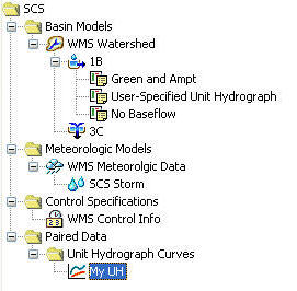 sing
the "real" unit hydrograph instead of using a synthetic unit hydrograph.
sing
the "real" unit hydrograph instead of using a synthetic unit hydrograph.
How to enter a user defined UH data in HMS.
1. In HMS, select Components | Paired Data Manager. Select the Data Type to be Unit Hydrograph Curves.
2. Click on New, change the name to My UH and click Create. Close the Paired Data Manager dialog.
3. Now expand the paired data in the watershed explorer window where you can see the UH you just created. Click on My UH. Then in the Data Editor window below it, select Paired Data tab. change the units to CFS and time interval to 15 mins (should be default).
4. Then
switch to Table tab and enter the hydrograph you got
from GSSHA simulation in part 2 above (i.e. the Unit Hydrograph ordinates
for 3 hour duration). The easiest way to do this is to open your hydrograph in Excel and then
cut/paste the hydrograph ordinates into HMS (a 15 minute time step will already
be defined). You can view your graph by switching to Graph tab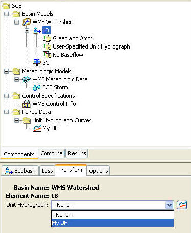 after all the data has been entered.
5. Now Click on the Watershed named 1B, (or different if you had renamed it) and go to transform tab. Select My UH for the Unit Hydrograph option. In sub basin and loss tabs, check if all data are entered properly.
The values should be
Sub basin: Loss method: Green and Ampt, Transform method: user specified Unit Hydrograph etc.
Loss: ( Initial content = 0.25 in, Saturated content = 0.45, suction = 12 in, Conductivity = 0.25 in/hr, Impervious = 0%)
6. Save your HMS project with new name and Run it.
You will compare the results for this simulation with the results from Assignment 21 1a,1b and Assignment 22 part 1(above).
-
Plotted hydrographs for each of the model runs above. Paste you outflow values into this template. (If you didn't use the correct write frequencies, you may have to adjust the charts in the template.)
To Turn in with Assignment 23 (think about these now):
-
Comparison between Variable and uniform roughness in GSSHA (and SCS and Clark methods in HMS.
-
Notes on numerical simulation methods.
-
Interception sensitivity analysis (remember not in the template)
-
Observations on your plots used to determine the time of concentration for the basin.
-
Comparison of variable roughness in GSSHA, SCS and Clark methods in HMS, and the results from using the GSSHA generated unit hydrograph in HMS.