Overview
As the flood hydrograph moves along a stream, it gets attenuated and lagged. The mathematical procedure used to simulate this phenomenon is called routing. There are basically two different routing techniques in stream flow which are hydraulic and hydrologic routing. In this assignment we will be using hydrologic routing. In the hydraulic routing technique, the St. Venant equation is solved. We will again use Judy's branch data for this assignment.
HEC HMS has different routing options built in the program like Kinematic wave method, lag method, Muskingum method, Muskingum Cunge etc. We will be using Muskingum and Muskingum Cunge and look at various options.
Model Set up
Use your basic Judy's branch WMS project with the SSURGO soil information.
Create an intermediate outlet so that there is one sub basin. You may want to redelineate (it is good to review periodically) and change the Threshold value to 0.1 (so that you have a denser river network which will be useful in further sections). Your basin schematic should look somewhat like this.
Create land use and soil type coverages in WMS and determine the curve number for the watershed as usual.
Processes
1. Muskingum Routing Method
In this part we will develop the Muskingum parameters based on the channel geometry and length.
a. Muskingum Parameter Estimation
Muskingum routing equation can be expressed as S = K [ XI + (1-X)O]
Where, S = Storage in the channel
K = Travel time of the flood wave through the reach
I = Rate of inflow to the routing reach
O = Rate of outflow from the routing reach
X = Dimensionless weighing factor ( 0 to 0.5, 0 means maximum attenuation and 0.5 means no attenuation or complete translation)
But in most of the cases the values of I and O are not available to determine the values of K and X. So Engineer Manual by the US Army Corps suggests a simplified method to determine these parameters. (For detail information you may see EM 1110-2-1417, Page 9-13 to 9-15).
To determine K
K = L/V
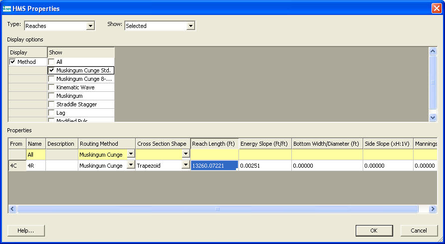
Where, L = Length of the routing reach in feet (WMS calculates this value. To see this value, double click the upper outlet and in routing method select Muskingum Cunge. Then the reach length is displayed there. See the following figure.
V = Flood wave velocity feet/sec (you can use WMS channel calculator to approximate the velocity based on the reference flow you use).
To determine X
Where, Q0 = reference flow from the inflow hydrograph (generally mid point between base flow and peak flow)
B = Top width of the flow area
S0 = Friction slope or bed slope (WMS calculates for you, go to display options and turn the display ON in drainage data, be sure you used the slope for lower sub basin).
C = Flood wave speed
Dx = Length of the routing sub reach = Total length of reach divided by the number of time steps
(WMS calculates total length of reach for you, go to display options and turn the display ON in drainage data, be sure you used the length for lower sub basin, Number of time steps is determined as given below)
Note: If your X is greater than 0.5, then there is some error in your calculation
To determine the number of time steps (or the number of sub reaches):
Number of Time steps = K/Dt
Where Dt = Computation time interval, 6 mins in this assignment
b. Model Run
Watershed: Two Basins
Loss Rate Method: Green and Ampt ( Initial loss = 0.3 in, Saturated Moisture =.45, Initial moisture = 0.25, suction = 12 in, Conductivity = 0.25, Impervious = 0%)
Transform method: Clark
Lag time: Kerby Method for Overland Flow for Tc
Precipitation: 2.5 inches with a Type II temporal distribution.
Model Run: 36 hrs @ 6 mins interval
You need to define the routing parameters for upper outlet. Switch to hydrologic modeling module, select the outlet selection tool
and double click the upper outlet. In the HMS properties window (as shown below) select the Routing method to be Muskingum. enter the values you determined for K and X
Now save the HMS file and run it in HMS.
c. Sensitivity of Muskingum Parameters
Change the values of both X and K as follows and rerun the model
Keep K constant and Change X as:
X = 0
X = 0.5
Keep X constant (original value) and Change K as: (Note as K changes the number of sub reaches will also change)
Increase by 50%
Decrease by 50%
Compare the results from b and c
2. Muskingum Cunge Routing Method
In this part we will use the Muskingum Cunge routing method and compare the results with the results from part 1 b.
a. Model Run
Watershed: Two Basins
Loss Rate Method: Green and Ampt ( Initial loss = 0.3 in, Saturated Moisture =.45, Initial moisture = 0.25, suction = 12 in, Conductivity = 0.25, Impervious = 0%)
Transform method: Clark
Lag time: Kerby Method for Overland Flow for Tc
Precipitation: 2.5 inches with a Type II temporal distribution.
Model Run: 36 hrs @ 6 mins interval
You need to define the routing parameters for upper outlet. Switch to hydrologic modeling module, select the outlet selection tool
Routing parameters:
Channel shape: Trapezoidal
Reach Length: Determined by WMS itself
Energy Slope: Determined by WMS
Bottom Width: 15 ft
Side slope: 2(H): 1(V)
Manning's n: Use the values you have been using for GSSHA assignments
Now save the HMS file and run it in HMS.
b. Sensitivity of Muskingum Cunge Parameters
Change the channel cross section to Deep and use side slope of 0(H): 1(V) and rerun the model
Compare the results from 2a with 2b
Compare the results from 2a with results from 1b
3. Comparison of two basin, 4 sub basins, 8 sub basins and MODClark
In this part we will compare the results from 1, 2, 4, and 8 basins models and MODClark and GSSHA models. For this comparison to work, we need to use the SCS curve number loss method and the Clark Transform Method for the multiple basin models. You already have most of these models built in one form or another from previous assignments, but you will need to change the loss method from Green and Ampt to SCS for some of them. Your 4 and 8 sub basin model should look somewhat like this and this.
Here is a summary of the models you should run and what settings you should use:
1, 2, 4, and 8 Basin Models:
Loss Rate Method: SCS Curve Number (using SSURGO soils) Make sure you calculate and specify the Initial Abstraction for each basin individually. (Ia = 0.2S and S = 1000/CN-10)
Transform method: Clark
Lag time: Kerby Method for Overland Flow for Tc
Precipitation: 2.5 inches with a Type II temporal distribution.
Model Run: 48 hrs @ 6 mins interval
Routing parameters: Muskingum Cunge with the same values as in part 2a above.
MODClark similar to (part 7 of assignment 18):
-
Loss Rate Method: Gridded SCS method (SSURGO soil)
-
Initial abstraction ratio 0.2, potential retention = 1.0.
-
Transform method: MODClark method
-
Tc and R-value: Kerby Method for Overland Flow for Tc
-
Precipitation: 2.5 inches with a Type II temporal distribution. Remember you must define this as a hyetograph.
-
Model Run: 48 hrs @ 6 mins interval
GSSHA:
-
Simply use the results from you GSSHA model which has spatially distributed Green and Ampt parameters based on the SSURGO Soil (Part 2 of Assignment 19).
You can create all of these models from scratch if you want, but it may be easier to modify existing models for the 1 and 2 basin and MODClark models. You will have to Create separate HMS models for 4 and 8 basins and enter the routing parameters as you did for two basins model.
To enter the
routing parameters, select the outlet selection tool
![]() and double click
on any outlets. In the properties window choose All for Show field and
select the routing method to be Muskingum Cunge in the box next to All (see
following figure). The values of Reach length and energy slopes are
calculated by WMS. Enter the same parameters for channel as you used for
part 2a for all the channels.
and double click
on any outlets. In the properties window choose All for Show field and
select the routing method to be Muskingum Cunge in the box next to All (see
following figure). The values of Reach length and energy slopes are
calculated by WMS. Enter the same parameters for channel as you used for
part 2a for all the channels.
Save HMS files and run for 4 and 8 basins models.
Compare the results from 1, 2, 4 and 8 basins, MODClark models, and GSSHA models.